Feature Level-Sets

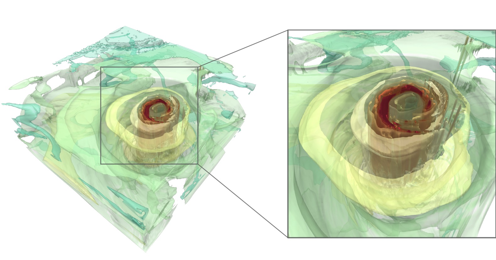
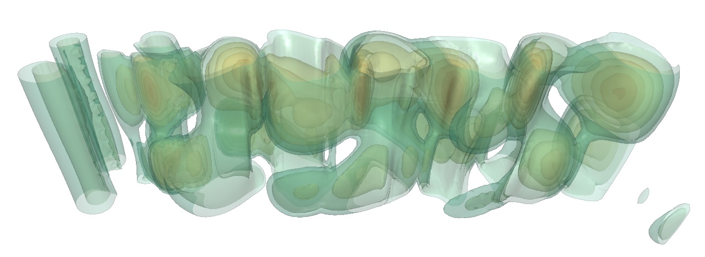
For an in-depth description of the method, I refer the interested reader to Feature Level-Sets: Generalizing Iso-surfaces to Multi-variate Data. Brief summary of the method: In a multivariate field, we treat every scalar field (or those we choose) as dimension of the attribute space. For example, if we consider a tensor field and calculate the three eigenvalues at every position we end up with three scalar fields; λ₁, λ₂, and λ₃, respectively. These three axes now define our attribute space. The next step is to define a geometry (or a set thereof) or even implicit function within this attribute space. We call this the trait. This trait should describe the parameter setup that we are looking for in the data. For example, if we look for regions where λ₁ is high and λ₃ is small (high anisotropy), we can define a point in the attribute space with those properties. Finally, for every data point in attribute space, we calculate the distance to this trait and transfer it back into its original physical location in the tensor field. After this process, we have a scalar field where at every position, the tensors’s distance towards the trait is stored. From this point on, we can use simple iso-surface rendering methods to display either regions that fullfil the sought-after criterion and/or level-sets thereof. This is particularly practical since the parameter configuration that we are looking for might not exists but we can still see, how “close” the tensor field gets to that configuration.
Contact: Jochen Jankowei
